Linear or Bilinear: A Criterion for Koopman Rollouts in Sampling-Based Predictive Control

Lee, Kangmin; Kim, Sanghyun

Abstract

The convention, and the criterion

Koopman operator models let sampling-based Model Predictive Path Integral (MPPI) control roll out thousands of sampled input sequences through an inexpensive learned lifted model. Existing Koopman-MPPI, however, keeps that lifted model linear in the input, a convention inherited from convex Koopman MPC that sampling never required. It fixes one input response for every configuration, and no criterion says when that is enough.

This paper supplies the criterion and builds the controller around it. When the configuration-dependent gain through which the input reaches the tracked output varies appreciably over the operating region, no constant input matrix can match it under the standard linear readout, no state dictionary repairs the mismatch, and a bilinear lift becomes necessary. When the gain is nearly constant, the two lifts predict alike. Since a bilinear step stays in the same matrix–vector cost regime either way, the criterion makes the bilinear model the default rollout.

Each sample's cost carries an online error tube from a proportional identification bound, and a free-energy analysis supplies a practical-stability guarantee. Across six systems, bilinear Koopman MPPI tracks with near-oracle accuracy on a wheeled vehicle and a drone under body-frame velocity commands, where its linear counterpart fails structurally. On force- and acceleration-driven platforms the two rollouts perform alike and bilinearity keeps mainly a parameter-efficiency advantage, which explains the successes reported for linear Koopman control.

See the criterion in action

Same lifting, two rollouts

The linear baseline and the bilinear controller share one deep Koopman lifting with identical network, training data, and multi-step loss. They differ only in the rollout equation. Whether that single change matters is a property of the robot, not the optimizer.

Linear ≈ bilinear: the gain barely varies

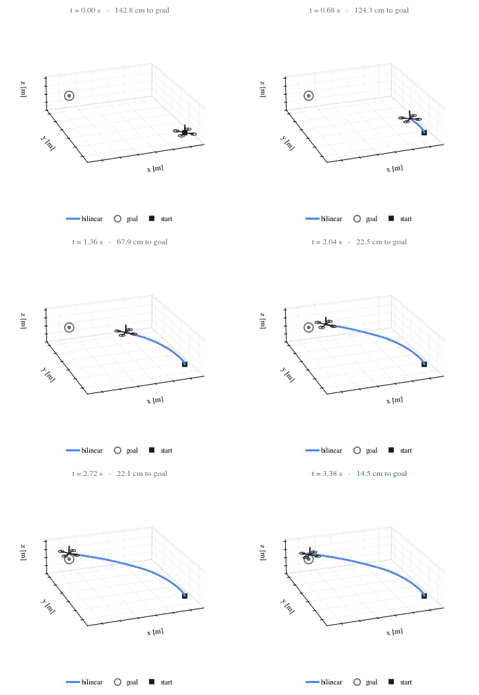
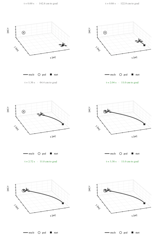
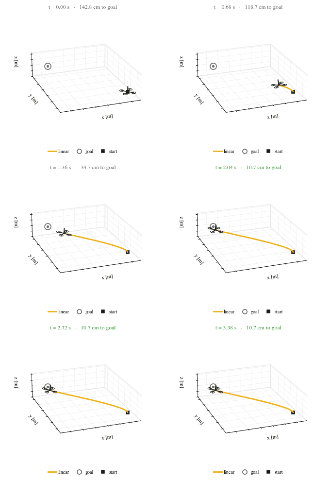
Thrust-driven quadrotor, fly-to-goal thrust command

Oracle

Linear

Bilinear

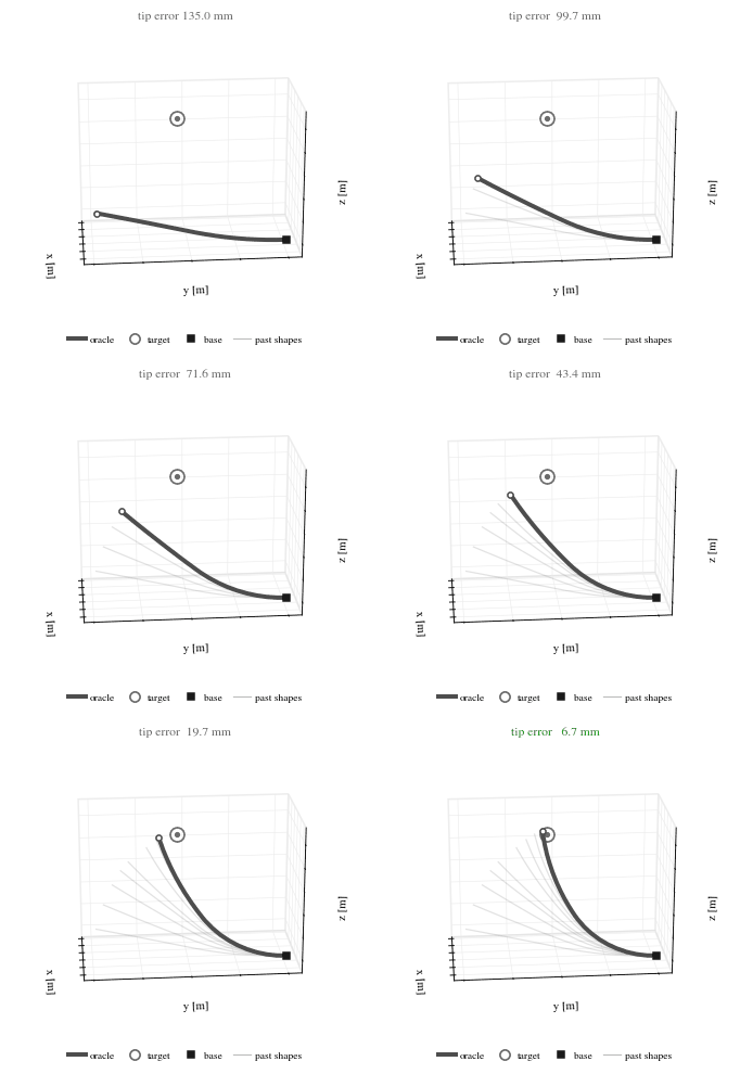
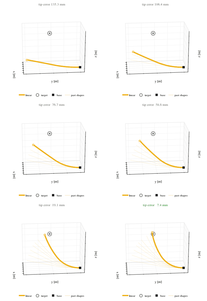
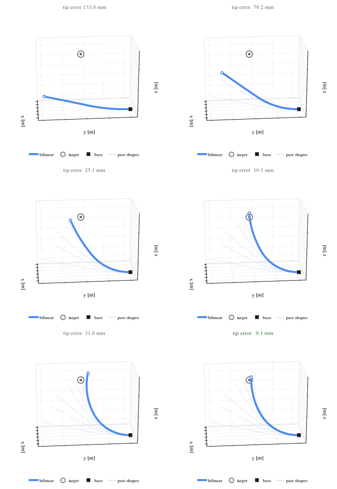
Cable-driven soft arm, reaching cable command

Oracle

Linear

Bilinear

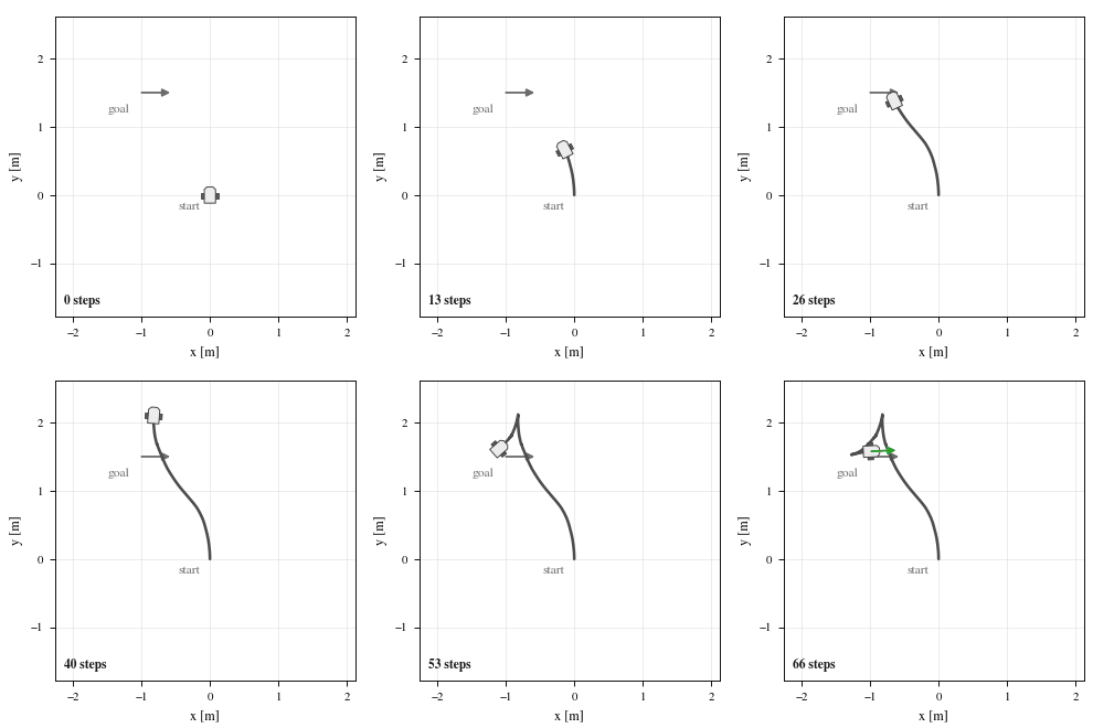
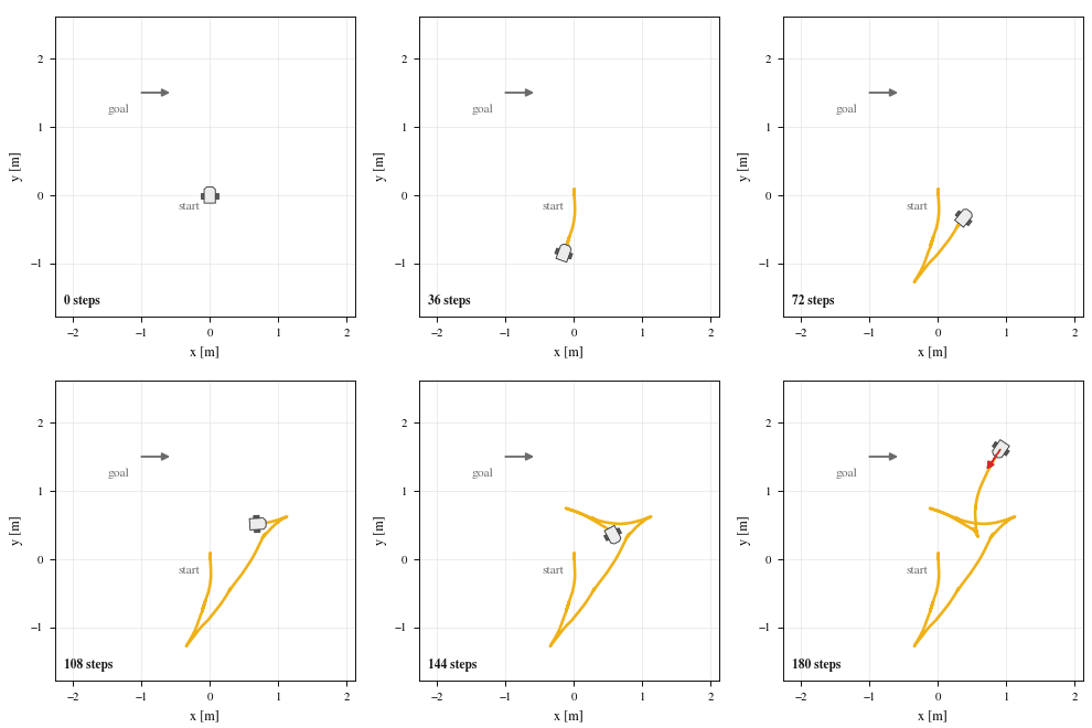
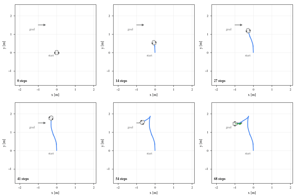
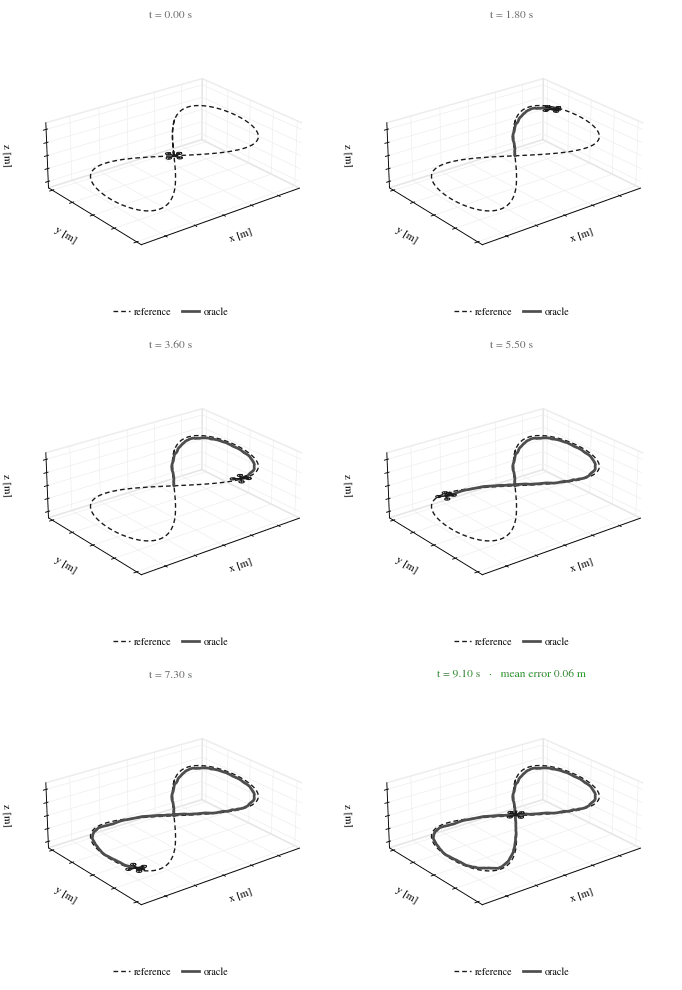
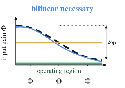
Bilinear necessary: the gain sweeps its range

Nonholonomic parking velocity command

Oracle

Linear

Bilinear

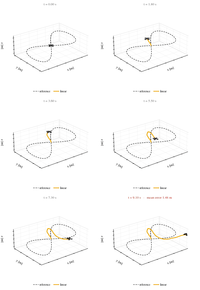
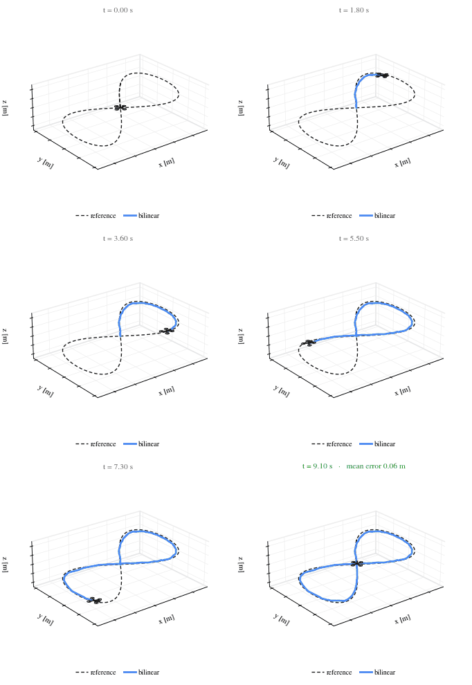
Body-velocity drone, figure-8 velocity command

Oracle

Linear

Bilinear

The failure is structural, not a lack of capacity. The linear rollout shares the bilinear model's network, data, and loss, and neither a larger lift nor a generic MLP closes the gap. When the input gain sweeps its range no constant input matrix can match it, and when the gain is nearly constant the two rollouts coincide. The dividing line belongs to the robot, not the optimizer.

Contributions

What the paper adds

A criterion for the rollout. A system-level test, the normalized gain variation ν̂, that decides when a Koopman-MPPI rollout must be bilinear and when a linear rollout suffices, as a property of the system rather than the optimizer.
Bilinear as the default. A bilinear Koopman MPPI controller built around the criterion, staying in the same matrix–vector rollout regime as the linear baseline (m+1 products per step, ~3.9 ms for K=1024).
Certified sample costs. An online error tube from a proportional identification bound carried in each sample's cost, with a free-energy practical-stability guarantee (0 violations over 82,000 held-out steps).
Evidence across six systems. The criterion is validated from velocity-commanded vehicles and drones, where the linear rollout fails structurally, to thrust- and force-driven platforms and soft arms, where the two rollouts coincide.

The criterion

When is bilinearity necessary?

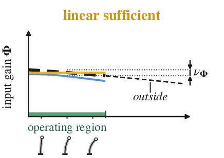
The distinction is a property of the system, not the optimizer. It is captured by the normalized variation of the input gain over the operating region.

ν̂ ≈ 0

The gain barely moves

Nearly constant input gain over the operating region

When the input reaches the output at second order (force, acceleration, torque) or the configuration barely turns, one constant input matrix fits the whole operating region. Linear and bilinear rollouts predict alike. This is the regime behind reported linear-Koopman successes.

ν̂ large

The gain sweeps its range

When a heading or yaw rotates the gain across its full range, no constant input matrix can match it under the linear readout, and no state dictionary repairs it, since the input matrix stays constant however wide the lift grows. Only a bilinear lift, where the input multiplies the lifted state, tracks the rotation.

Method

One lifting, two rollouts

Koopman lifts the state through a dictionary into z = Ψ(x), and MPPI rolls thousands of sampled input sequences through the lifted model. The whole question is how the input u enters that rollout.

Linear rollout

z⁺ = A z + B u

One constant input matrix B for every configuration, the convention inherited from convex Koopman MPC.

Bilinear rollout

z⁺ = A z + B₀ u + Σ_i u_i (B_i z)

The input also multiplies the lifted state, so the input response changes with configuration.

The tracked output is read back linearly, y = C_h z. Writing M(u) = A + Σ_i u_i B_i, the bilinear step becomes z⁺ = M(u) z + B₀ u: only m+1 matrix–vector products, the same rollout regime as the linear model. Both are identified from data by least squares or a jointly trained deep dictionary, and the bilinear form simply adds the products u_i z to the regressor. When the input gain varies over the operating region no constant B can match it, a bound that holds for any dictionary, so the bilinear term is necessary; when the gain is nearly constant the two coincide.

Bilinear Koopman MPPI · one control step

Lift the current state once, z₀ = Ψ(x).
Sample K input sequences V^(k) = U + ε^(k), with ε ∼ 𝒩(0, Σ).
Roll each through the bilinear model z⁺ = M(v) z + B₀ v, accumulating the trajectory cost S(V^(k)).
Update the plan: u_t ← u_t + (Σ_k w^(k) ε_t^(k)) ∕ (Σ_j w^(j)), w^(k) = exp(−(S^(k) − ρ) ∕ λ).
Apply u₀, shift U, and warm-start the next control step.

Results

Six systems, one dividing line

Each system is placed by its normalized gain variation ν̂. Where ν̂ is large the bilinear rollout is decisive; where ν̂ ≈ 0 the two coincide and only a parameter-efficiency edge remains.

System	Gain variation ν̂	Closed loop (Oracle / Linear / Bilinear)	Prediction: bilinear vs. linear
Unicyclevelocity command	R(θ), maximal (2.0)	92 / 0 / 84 % parked	42–48×	bilinear
Dronevelocity command	R(ψ), maximal (2.0)	0.05 / 1.4 / 0.05 m	135 ± 7×	bilinear
Pendulum	second order (0)	—	~4× fewer neurons	alike
Quadrotorthrust command	second order (0)	0.12 / 0.44 / 0.45 m	1.0–1.1×	alike
Torque arm	second order, inertia (0)	—	0.88–0.98×	alike
Soft arm	low (curvature)	—	0.93–1.09×	alike

Closed-loop entries: parking rate (unicycle), mean tracking error (drone), median goal distance (quadrotor). A prediction ratio near 1× means the two rollouts coincide; dashed rows are evaluated through prediction. Oracle rolls out the true dynamics and is not a performance ceiling.

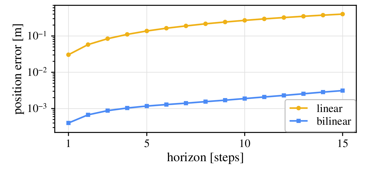
Drone: open-loop prediction

World-position error over the planning horizon (log scale). The gap is structural: doubling the linear lift's dimension does not close it.

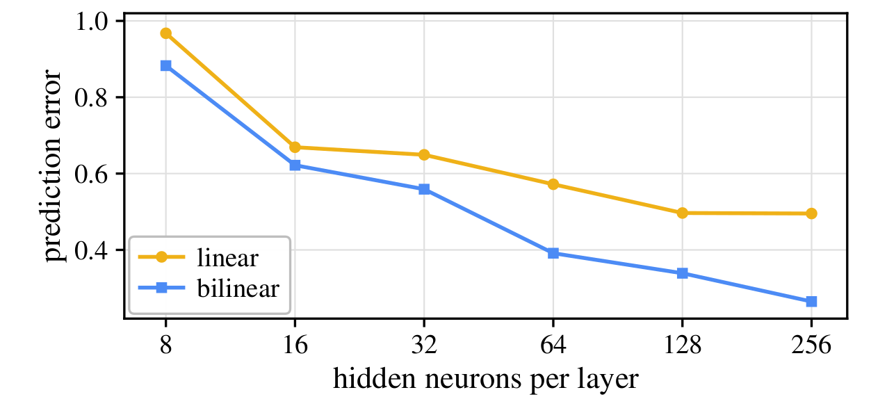
Pendulum: efficiency where coupling is weak

Even when bilinearity is not required, the structured input term substitutes for network width, matching linear accuracy with ~4× fewer neurons.

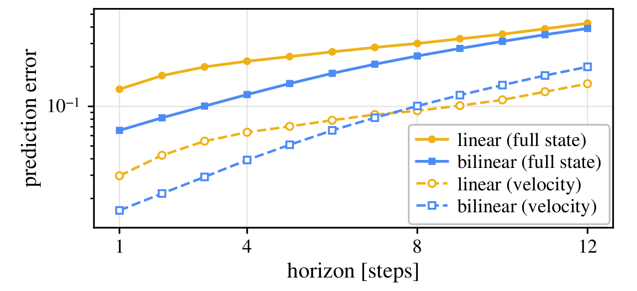
Quadrotor: the boundary

Thrust reaches position only through acceleration, so despite ±69° tilts the linear and bilinear predictions coincide on full state and velocity alike.

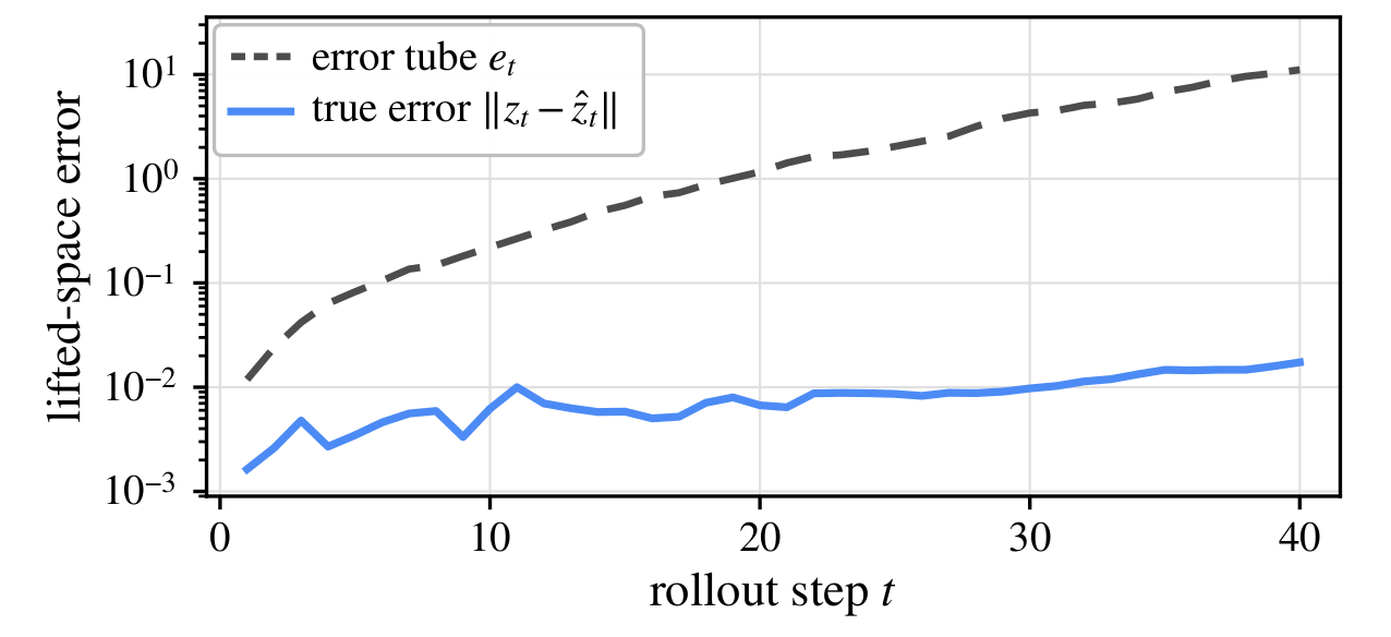
Error tube: 0 violations / 82,000 steps

Each sample's cost carries an online error tube from a proportional identification bound. It contains the true lifted error at every held-out step.

Ruling out capacity

Open-loop 15-step world-position error on the drone, mean ± s.d. over ten training runs on a shared 1,000-trajectory held-out set. A larger linear lift and a generic MLP both miss the rotation the bilinear lift represents exactly.

Rollout model	Latent N	Prediction error (m)
Linear	13	0.409 ± 0.001
Linear (large)	29	0.409 ± 0.001
MLP dynamics	—	0.078 ± 0.017
Bilinear	13	0.0030 ± 0.0001

Reproducibility

Experiment parameters

Key per-system MPPI hyperparameters, shared by the bilinear controller and the linear baseline. Method-specific choices follow the linear baseline's reported settings.

System	N (lifted dim)	K (samples)	T (horizon)	Δt (s)	λ (temperature)
Unicycle	8	1,536	40	0.05	0.4
Drone	13	1,024	15	0.05	0.25
Pendulum	8	2,560	65	0.05	0.8
Quadrotor	24	1,500	20	0.02	0.5

Simulators. Unicycle & drone kinematic · pendulum analytical · quadrotor & torque arm in MuJoCo · soft continuum arm in SoftManiSim

Protocol. Unicycle 50 parking trials · drone 60 episodes · quadrotor 20 runs

Rollout cost. m+1 matrix–vector products per step vs. 1 for linear, the same cost regime

Timing (CPU, 4 threads). 3.9 ms bilinear vs. 13 ms true-dynamics vs. 76 ms physics-engine rollout

Citation

BibTeX

@article{lee2026linearbilinear,
  title   = {Linear or Bilinear: A Criterion for Koopman Rollouts
             in Sampling-Based Predictive Control},
  author  = {Lee, Kangmin and Kim, Sanghyun},
  journal = {International Journal of Control, Automation and Systems},
  year    = {2026},
  note    = {Under review},
  url     = {https://rcilab.github.io/koopman-mppi}
}